Three principles for epidemic dynamics

How to get quick insights into importations, transmission and reporting

Something happens when you work on a topic for many years. Along the way, you pick up little nuggets of insight – rules and principles that can give ideas about what will happen, even if you don’t do a detailed analysis.

When it comes to thinking about large epidemics – whether dengue, Zika, influenza or COVID Omicron variants – I’ve found there are three handy principles about how key factors will change the resulting dynamics. 

Principle 1: Initial infections shift the epidemic curve sideways

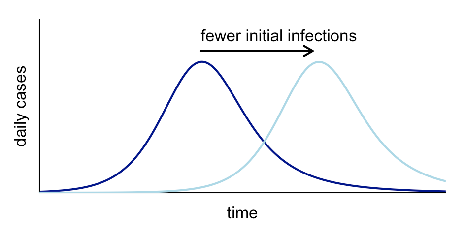
Assuming there are enough imported infections for a large epidemic to take hold in a location, we’d generally expect the number of initial imported cases to change the timing of the epidemic, but not its shape:

Mathematical explanation (for those who’re interested): Early epidemic growth typically follows an exponential process (because infections lead to more infections that lead to more infections). This can be written as a*exp(g*t), where a is the number of initial infections, g is the growth rate and t is time. Because an exponential process (i.e. the local epidemic) grows much faster than a linear one (i.e. the number of initial infections), any change in imported infections pales in comparison to the number of new infections that will soon be generated locally. Hence fewer imported infections delay the curve, rather than changing its shape. (The exception would be if transmission is strongly seasonal, and delayed introduction starts the epidemic in the high/low transmission season instead).

Principle 2: Transmission rate changes the slope and peak

The transmission rate affects the slope of the curve and its overall height (in the scenario where the epidemic ends because of accumulation of immunity). If the transmissibility of the infection is lower, the epidemic trajectory will increasingly diverge from the higher transmission scenario, leading to a lower peak:

Mathematical explanation: If exp(g*t) is the curve with baseline growth rate g, and exp(h*t) represents the curve for a lower growth rate h, where h < g, then the ratio of the two growth curves will be equal to exp((g-h)*t), and hence the gap between the curves will grow exponentially during the early period of the epidemic. The peak will be lower because for epidemics that end because of accumulation of immunity – like dengue, Zika and influenza – the level of susceptibility at the peak, and hence the number of new infections being generated at this point, is inversely proportional to the magnitude of transmission.

Principle 3: Case reporting scales the curve vertically

If a smaller proportion of infections are reported, it won’t change the timing or slope of the epidemic curve, but it will scale down the curve proportionally. E.g. if the proportion of infections reported as cases in the surveillance system drops from 50% to 25%, it will cut the height of the observed peak in half:

Mathematical explanation: During a large epidemic of an infection like influenza or dengue, the process of reporting individual infections typically doesn’t trigger actions that will have a strong impact on the process of transmission itself (unlike outbreaks like Ebola, where identification of cases will lead to contact tracing, and hence disrupt transmission). If fewer infections are reported as cases during a large epidemic, it will therefore scale the number of observations linearly, but the underlying epidemic dynamics will remain the same.

Why are these ideas useful?

Often there is speculation about why epidemics look different across various locations or time periods. The above principles can be useful for thinking about whether the likely cause is the number of initial imported cases, the extent of reporting, or variation in transmission itself.

These principles can also help us understand what we can realistically estimate from available data. For example, if only a fraction of infections are reported, but this fraction is reasonably consistent over time, we can still estimate the extent of transmission and pattern of introduction because reporting doesn’t affect the growth rate or timing of the peak.

What’s more, these concepts can help in sense checking new analysis. Suppose someone makes a claim about how differences in transmission or imported cases will change the shape of an epidemic. Or they generate scenarios with different assumptions about how many cases are being reported. Having simple rules-of-thumb available lets people perform some quick plausibility checks without having to run the full simulations themselves.

On numerous occasions when reviewing new results or papers , I’ve used these three principles to spot potential flaws in analysis – or opportunities for better explanations. So I’m sharing here in the hope that they might help others spot them too.